Getting started

This web page can be downloaded as notebook: schroedinger_cat.ipynb (Jupyter) or schroedinger_cat.md (Markdown)

This tutorial demonstrates the basic setup of a Wavepacket calculation, and of the core features: Switching between wave functions and density operators with minimal overhead

General setup

For this tutorial, we only consider a one-dimensional free particle. More complex setups are possible, see other tutorials and advanced demos.

As general setup, we need to do two things:

Set up a grid / basis expansion for your system. A (multidimensional) “grid” is the direct product of one-dimensional grids, called “degrees of freedom” (DOF) in Wavepacket. Note that Wavepacket uses exclusively the DVR / pseudo-spectral method, see Representation of states or the wiki[1] for details.
Given a grid, define relevant operators. Here, we only need a Hamiltonian, but in other settings, you might also want to calculate expectation values of other operators, for example.

import wavepacket as wp

# 1. One-dimensional grid with a plane wave expansion DOF == equally-spaced grid
dof = wp.grid.PlaneWaveDof(-20, 20, 128)
grid = wp.grid.Grid(dof)

# 2. The Hamiltonian consists of only the kinetic energy p^2/2m.
hamiltonian = wp.operator.CartesianKineticEnergy(grid, 0, mass=1.0)

A few notes about the code so far:

Wavepacket makes heavy use of immutable objects. Every object in Wavepacket is defined on construction and should not be modified later. This pattern avoids unintended, surprising side effects from modifying objects used already elsewhere. Note, though, that the Python interpreter does not always enforce this immutability, only IDEs or static checkers will complain.
For multidimensional grids, just supply a list of DOFs instead of a single DOF, e.g., wp.grid.Grid([dof, dof]). We use this pattern of applying either a single object or a list of objects extensively where one or multiple objects can be supplied.
We tried to keep the interfaces consistent where possible. For example, all operators take the grid as first parameter, followed (where it makes sense) by the index of the dimension along which the operator acts, followed by other parameters.

Operators themselves are sometimes used directly, for example when diagonalizing an operator or propagating in imaginary time. Usually, however, you wrap them into an Expression to specify which equation of motion you want to solve.

Evolving wave functions in time

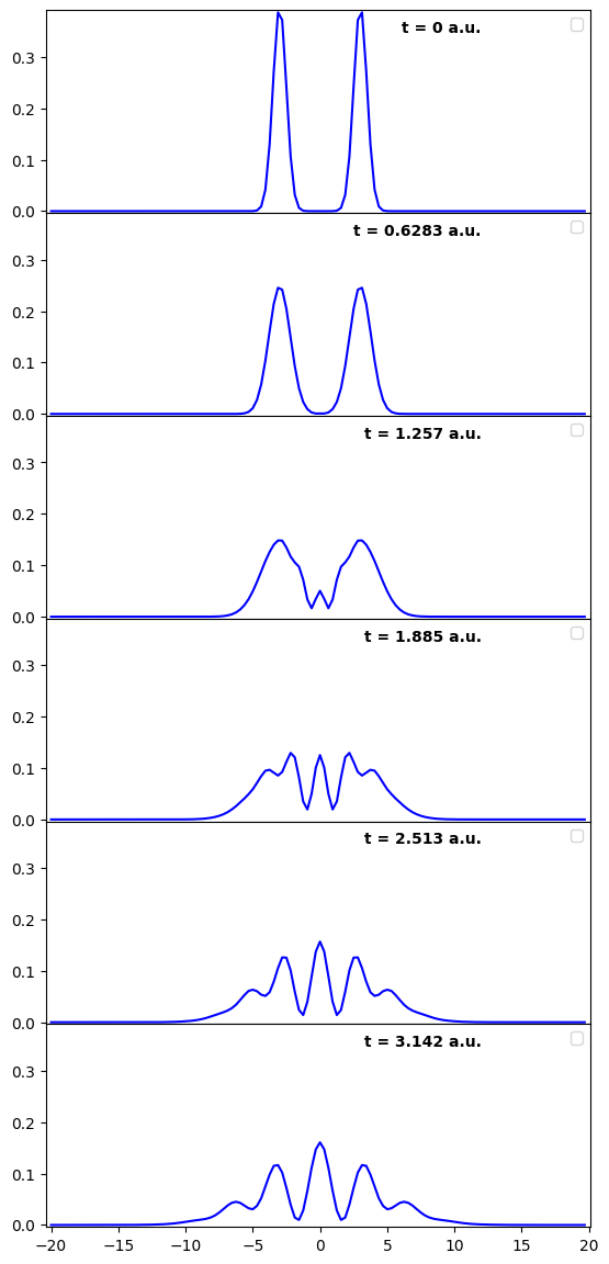
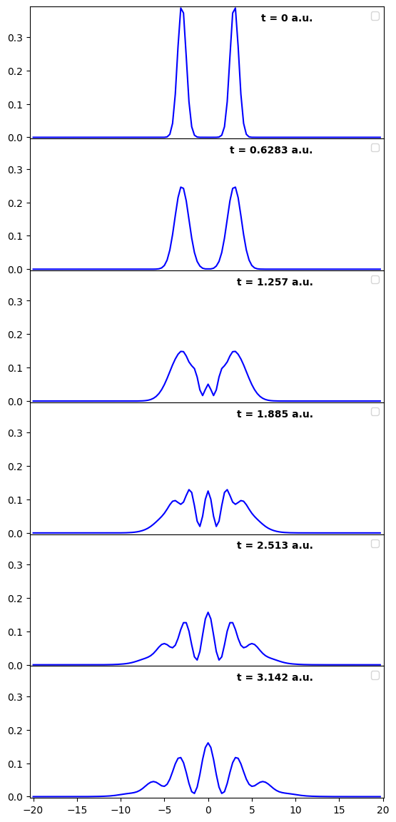
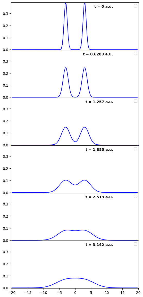
Let us first evolve some wave packet in time. To produce non-trivial dynamics, we prepare a “Schrödinger cat state” with two interfering Gaussian wave packets, $\psi = 1/\sqrt{2} (\psi_L + \psi_R)$ .

For the wave function setup, we need to:

set up the initial wave function
define the (Schrödinger) equation of motion to solve
set up a solver for the time evolution.

Of course, once we propagate our state in time, we want to do something with the result. Here, we just plot the density.

import math

rms = math.sqrt(0.5)
psi_left = wp.builder.product_wave_function(grid, wp.special.Gaussian(-3, rms=rms))
psi_right = wp.builder.product_wave_function(grid, wp.special.Gaussian(3, rms=rms))
psi_0 = math.sqrt(0.5) * (psi_left + psi_right)

schroedinger_eq = wp.expression.SchroedingerEquation(hamiltonian)
solver = wp.solver.OdeSolver(schroedinger_eq, dt=math.pi/5)

plot_1d = wp.plot.StackedPlot1D(6, psi_0)
for t, psi in solver.propagate(psi_0, t0=0.0, num_steps=5):
    plot_1d.plot(t, psi)

../_images/b38190174f7a721d5f21d5eb4911b0f02d03f78972616610574a4748fe919b1f.png

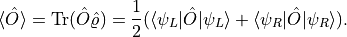
As can be seen, as soon as the wave packets encounter each other, we get typical oscillations. This is easily understood because any observable, such as the density at a given point, is calculated as

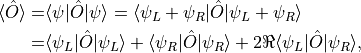
$\begin{align*} \langle \hat O \rangle =& \langle \psi | \hat O | \psi \rangle = \langle \psi_L + \psi_R | \hat O | \psi_L + \psi_R \rangle \\ =& \langle \psi_L | \hat O | \psi_L \rangle + \langle \psi_R | \hat O | \psi_R \rangle + 2 \Re \langle \psi_L | \hat O | \psi_R \rangle , \end{align*}$

where the last term causes the interferences, and distinguishes quantum mechanics from simple ensemble averaging.

The result of constructing a wave function or of a propagation is a wavepacket.grid.State object. These objects hide the difference between wave functions and density operators, and they are bound to a specific grid. You should rarely ever need to deal with the internals of this class, because almost all Wavepacket functionality takes or outputs a state.

Wavepacket tries to abstract away differences between wave functions and density operators where possible. As one example, Wavepacket does not offer a function to calculate the norm, because the L2-norm for wave functions is a different quantity than the trace norm for density operators, which is highly confusing (at least it confused me repeatedly). Wavepacket therefore offers a function to calculate the trace, which has the same definition for both types of states.

Here, we used a simple ODE solver that employs a slow but robust Runge-Kutta procedure by default. Again, solvers have a consistent interface that takes the expression as first parameters, followed by the time step and all other parameters.

Instead of just plotting the result, you might wish for more advanced processing. See Pendular states for a more elaborate example.

Evolving density operators in time

One of the strengths of Wavepacket is the minimum overhead switch to a density operator formalism. We use almost the same setup as for wave functions case except for two changes: Our initial state is a density operator, not a wave function. And we set up a Liouville von Neumann equation (LvNe); for a closed system, this is just the commutator with the Hamiltonian.

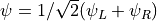
To contrast density operator dynamics with wave function dynamics, we set up an incoherent sum of the left and right Gaussian wave packets, $\hat \rho = 1/2 (|\psi_L\rangle\langle\psi_L| + |\psi_R\rangle\langle\psi_R|)$ .

rho_0 = 0.5 * (wp.builder.pure_density(psi_left) + wp.builder.pure_density(psi_right))

liouvillian = wp.expression.CommutatorLiouvillian(hamiltonian)
solver = wp.solver.OdeSolver(liouvillian, dt=math.pi/5)

plot_1d = wp.plot.StackedPlot1D(6, rho_0)
for t, rho in solver.propagate(rho_0, t0=0.0, num_steps=5):
    plot_1d.plot(t, rho)

../_images/c56c493e4a2e3adbf4ee6811eb5cc3d2eacc20738ff53cd79308b0c318f9423a.png

Now we see no interference terms anymore, because we only get the ensemble average,

$\langle \hat O \rangle = \mathrm{Tr} (\hat O \hat \varrho) = \frac{1}{2} ( \langle \psi_L|\hat O |\psi_L \rangle + \langle \psi_R| \hat O |\psi_R\rangle) .$

If we choose the direct product of the initial wave function (coherent summation), we recover the oscillations, of course.

rho_0 = wp.builder.pure_density(psi_0)
plot_1d = wp.plot.StackedPlot1D(6, rho_0)
for t, rho in solver.propagate(rho_0, t0=0.0, num_steps=5):
    plot_1d.plot(t, rho)

../_images/7017c2965a19a36957f4f8586364d83caf19d9d27fb7b5a3635b498549bac916.png