Background theory: ODE solvers

This web page can be downloaded as notebook: ode_solvers.ipynb (Jupyter) or ode_solvers.md (Markdown)

Here, we want to have a look at conventional ODE solvers. In particular, how do you check calculations, and how do you speed up a calculation?

For the impatient, the main results of the following treatise are:

Poor convergence can show up as a divergent norm. In practice, however, ODE solvers use adaptive step sizes; for reasonable parameters, they just take forever.
The required time step, hence the performance, is dictated by the largest (absolute) eigenvalue, not by the typical energies.
Truncate aggressively and shift energies to improve performance.

Some basics

ODE solvers theory

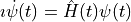
We start from the Schrödinger equation

$\imath \dot \psi(t) = \hat H(t) \psi(t)$

and expand the wave function in a complete basis with time-dependent coefficients, $|\psi(t)\rangle = \sum_n c_n(t) |\phi_n\rangle$ . Inserting and multiplying with $\langle \phi_m |$ gives the formula for the coefficients,

$\imath \dot c_m(t) = \sum_n \langle \phi_m| \, \hat H \, |\phi_n \rangle \ c_n(t)$

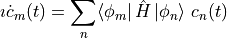
This is a system of ordinary differential equations, and any explicit solver can be used for the time evolution, most notably Runge-Kutta algorithms. A similar derivation can be done for the Liouville von-Neumann equation for density operators.

ODE solvers have the big advantage that they are robust work horses. You can throw any problem at them: time-dependent Hamiltonians, complex-valued Hamiltonians, open systems, … they will produce a solution. Nowadays, they always come with adaptive time steps, so you only need to set an error bound, and the algorithm chooses an appropriate time step for you.

The big drawback is performance; ODE solvers do not exploit any knowledge of the system, and this makes optimized solvers like polynomial solvers more efficient for specific classes of problems. Typically, ODE solvers are not unitary, so the norm is not a conserved quantity and diverges on poor convergence. However, because of the adaptive steps, this does not usually happen, instead the algorithm chooses tiny step sizes with corresponding long run times.

Model system

As example system, we choose a one-dimensional harmonic oscillator with a shifted Gaussian as initial state.

import wavepacket as wp

grid = wp.grid.Grid(wp.grid.PlaneWaveDof(-10, 10, 128))
hamiltonian = (wp.operator.CartesianKineticEnergy(grid, 0, 1.0)
              + wp.operator.Potential1D(grid, 0, lambda x: 0.5 * x ** 2))
equation = wp.expression.SchroedingerEquation(hamiltonian)

psi0 = wp.builder.product_wave_function(grid, wp.special.Gaussian(x=-3, rms=2))

Let us have a look at the projection onto the Hamiltonian eigenstates:

import matplotlib.pyplot as plt
import numpy as np

eigenstates = [state for _, state in wp.diagonalize(hamiltonian)]
projection = [wp.population(psi0, state) for state in eigenstates]

plt.semilogy(np.arange(128), projection, '+');

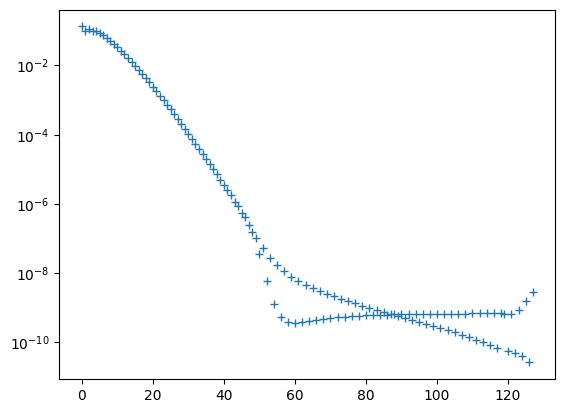
../_images/fa3ff034fd4b5b4f21a1aa15cfb5816de2ae0c4ae01f4108ceeca6219c6e802c.png

In theory, the population should decay smoothly. In practice, strange things start to happen around the 50th eigenstate. If we play around with the grid parameters, it can be shown that this is an artifact of the finite grid extent and the finite number of grid points. We skip the demonstration here to reduce the run time of the notebook. This finite grid error is a common issue and discussed in depth in Background theory: Converging equally-spaced grids.

Convergence behavior

Intuitively, we would assume that the time step is determined by the specific dynamics, i.e., the initial wave function for our time-independent system. For example, a low-energy state evolves slower in time than a high-energy state, hence it should allow larger time steps. Unfortunately, this intuition is incorrect.

To understand what happens let us force a calculation to not converge. This is a contrived example; scipy’s ODE solvers always use adaptive stepping, so we need to choose absurd parameters to render this mechanism ineffective. To understand where exactly things go awry, we can plot the populations of the individual eigenstates

solver = wp.solver.OdeSolver(equation, 0.1, atol=1e10, first_step=0.01)
x = np.arange(128)

for t, psi in solver.propagate(psi0, 0, 2):
    print(f"t = {t}      Trace = {wp.trace(psi)}")

    populations = [wp.population(psi, state) for state in eigenstates]
    plt.semilogy(x, populations, '+')

t = 0      Trace = 1.0
t = 0.1      Trace = 108.80646924606806
t = 0.2      Trace = 2577050522990.972

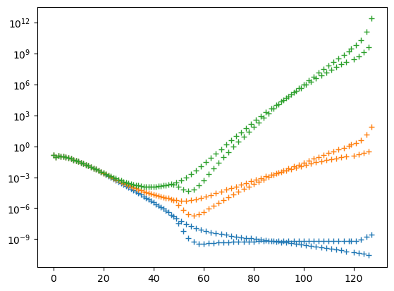
../_images/3003b9c30f729707be12d4d2f0f8485d4d2cc2a5b1459dc75f279bd84a8f9b60.png

We succeed: The norm diverges rapidly. From the plot of the populations, we find that the divergence is caused only by the high-energy contributions. These are completely irrelevant for the actual dynamics, but require small timesteps for accurate time evolution.

Improving the efficiency thus require an optimization of the operator spectrum. There are two options: We can shift the spectrum, or we can truncate it.

Shifting the spectrum

The solver spends most effort on the correct propagation of the populated states with the highest energies. This burden can be reduced by shifting the operator spectrum, thereby making the largest (absolute) energies smaller. Simple scaling laws suggest that the required time step scales with the inverse of the largest energy, so shifting the spectrum to be balanced around zero would ideally halve the computation time.

To see what happens, let us repeat the previous analysis with the spectrum shifted by 50 atomic units (approximately the energy of the 50th eigenstate)

shifted_equation = wp.expression.SchroedingerEquation(hamiltonian - 50)

shifted_solver = wp.solver.OdeSolver(shifted_equation, 0.1, atol=1e10, first_step=0.01)
x = np.arange(128)

for t, psi in shifted_solver.propagate(psi0, 0, 2):
    print(f"t = {t}      Trace = {wp.trace(psi)}")

    populations = [wp.population(psi, state) for state in eigenstates]
    plt.semilogy(x, populations, '+')

t = 0      Trace = 1.0
t = 0.1      Trace = 25.81214582656713
t = 0.2      Trace = 5795695256.290543

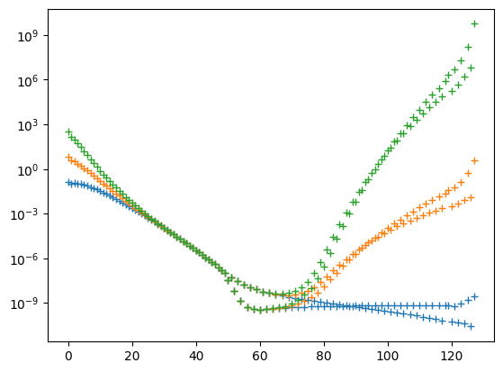
../_images/08d63117fa1d9c4343ecd9c134865c1f8c606016a5a73c52e283b80c4c76212f.png

The good news is that the shift helps visibly with the divergent trace. Alas, now the populations of the low-energy eigenstates start to diverge. This causes problems with adaptive step sizes, because the low-energy eigenstates have larger populations, therefore they contribute more to the step error.

As a consequence, shifting by half of the spectral range is probably not optimal. To figure out the optimal value, we use a “Counting expression” that measures how often our Hamiltonian is applied, which is the expensive part of the algorithm.

class CountingExpression(wp.expression.ExpressionBase):
    def __init__(self, wrapped_expression):
        super().__init__(False)

        self._wrapped_expression = wrapped_expression
        self.count = 0

    def apply(self, state, t):
        self.count += 1
        return self._wrapped_expression.apply(state, t)

Then we can try out the computational effort for different energy shifts:

for shift in range(0, 51, 10):
    shifted_equation = wp.expression.SchroedingerEquation(hamiltonian - shift)
    counter = CountingExpression(shifted_equation)
    solver = wp.solver.OdeSolver(counter, 0.5)

    solver.step(psi0, 0)
    print(f"Shift = {shift} a.u.      count = {counter.count}")

Shift = 0 a.u.      count = 374
Shift = 10 a.u.      count = 356
Shift = 20 a.u.      count = 338
Shift = 30 a.u.      count = 314

Shift = 40 a.u.      count = 302
Shift = 50 a.u.      count = 356

We find an optimal shift of around 40 a.u., which reduces the computational effort by about 25%, only half the maximum possible reduction. The drawback of this shifting is the required guesswork to find a suitable energy shift; after all computing time is often cheaper than the scientist’s attention. And choosing the time step suboptimally yields even smaller gains.

Truncating the spectrum

The second manipulation is a direct truncation of the operator spectrum. While this may appear clumsy, there are good reasons to truncate aggressively:

As the previous analyses have shown, high-energy eigenstates are poorly represented by the grid anyway. In the example here, this affects everything above about the 50th eigenstate. Aggressive truncation therefore only invalidates results that were already incorrect in the first place.

In theory, we could remove these artifacts by extending the grid, but then we pay twice: The larger grid makes all computations slower, and to faithfully propagate the large-energy components, we need smaller time steps. And at the end of the day, the gain in accuracy is tiny. because the populations of the high-energy eigenstates are small, after all.
Whenever we simulate existing physical systems, we use models. These models are always low-energy approximations of the real system. For example, we neglect anharmonic contributions, or we ignore the coupling to highly excited electronic states, maybe we even ignore excited states entirely within the Born-Oppenheimer approximation. In the particular example here, we can safely assume that the 50th excited state will be anything but a harmonic eigenstate.

Again, this means that by truncating the Hamiltonian, we merely trade one incorrect approximation for another, so no harm is done.

Truncating the spectrum of the Hamiltonian requires an expensive diagonalization, so we truncate the individual components instead.

Similar to the shifting of the spectrum, we can study the effect of truncation on the efficiency.

for cutoff in range(50, 201, 50):
    truncated_hamiltonian = (wp.operator.CartesianKineticEnergy(grid, 0, 1.0, cutoff=cutoff)
                            + wp.operator.Potential1D(grid, 0, lambda x: 0.5 * x ** 2, cutoff=cutoff))
    truncated_equation = wp.expression.SchroedingerEquation(truncated_hamiltonian)
    counter = CountingExpression(truncated_equation)
    solver = wp.solver.OdeSolver(counter, 0.5)

    solver.step(psi0, 0)
    print(f"Cutoff = {cutoff} a.u.      count = {counter.count}")

Cutoff = 50 a.u.      count = 158
Cutoff = 100 a.u.      count = 236
Cutoff = 150 a.u.      count = 314
Cutoff = 200 a.u.      count = 368

The computational effort drops considerably when reducing the cutoff, which supports the thesis that significant effort is spent on propagating high-energy contributions. After truncating the kinetic and potential energy to 50 a.u. each, we are left with less than half of the original computational effort. If we show more restraint and truncate only at 100 a.u., we still reduce the computational effort by one third. These numbers suggest an advantage of truncation: Even suboptimal or cautious guesses reduce the computational effort significantly.

How bad is the approximation for the dynamics? To answer this question, we can look at the projection of the truncated result on the untruncated result; any deviation from one can serve as a figure of merit of the additional error.

import math

truncated_hamiltonian = (wp.operator.CartesianKineticEnergy(grid, 0, 1.0, cutoff=50)
                        + wp.operator.Potential1D(grid, 0, lambda x: 0.5 * x ** 2, cutoff=50))
truncated_equation = wp.expression.SchroedingerEquation(truncated_hamiltonian)
truncated_solver = wp.solver.OdeSolver(truncated_equation, math.pi / 2)
truncated_result = truncated_solver.step(psi0, 0)

solver = wp.solver.OdeSolver(equation, math.pi/2)
result = solver.step(psi0, 0)

print(f"Overlap after pi/2: {wp.population(truncated_result, result)}")

Overlap after pi/2: 0.9999936604721268

The additional deviation in the sixth decimal is of a similar magnitude and therefore consistent with the grid error, so we have introduced no undue additional approximation.