Pendular states

This web page can be downloaded as notebook: pendular_states.ipynb (Jupyter) or pendular_states.md (Markdown)

The goal of this demo is the partial reproduction of some results of a paper by Ortigoso et al.[1] Besides discussing pretty cool physics, it aims to demonstrate how to extract non-trivial data with minimal fuss and plot it.

Alignment of molecules, some theory

If a molecule interacts with a non-resonant laser field, the electronic ground state is shifted in energy. We can calculate the shift with standard perturbation theory and cavity-dressed states as

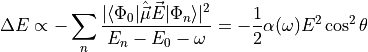
$\Delta E \propto - \sum_n \frac{|\langle \Phi_0 | \hat{\vec{\mu}} \vec E |\Phi_n \rangle|^2}{E_n - E_0 - \omega} = - \frac{1}{2} \alpha(\omega) E^2 \cos^2 \theta$

in terms of the dipole operator $\mu$ , the electric field with strength $E$ and frequency $\omega$ , and where the summation includes all excited states $\Phi_n$ with energies $E_n$ . Calculating the energy shift is difficult, but that is not our goal here. Instead, we absorb all these calculations in a material-specific dynamic polarizability $\alpha(\omega)$ . Then only a dependency on the angle $\theta$ between the effective dipole moment and the laser polarization axis remains.

If we plug this energy shift into the formula of a rigid linear rotor, we arrive at the Hamiltonian

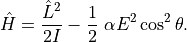
$\hat H = \frac{\hat{L}^2}{2I} - \frac{1}{2} \ \alpha E^2 \cos^2\theta.$

This Hamiltonian describes a linear rotor (first term) trapped in a cosine-shaped potential that draws the rotor towards the laser polarization axis ( $\alpha > 0$ ) or away from it ( $\alpha < 0$ ). In the following, we only consider the former case of a positive polarizability. As the final step, we introduce three further manipulations:

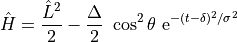
We assume that the electric field changes slowly (adiabatically) over time. Effectively, this adds a time-dependent shape function to the second term in the Hamiltonian. We will follow the reference and assume a Gaussian shape.
Because only the product of electric field strength and polarizability matters, we replace it by a single parameter.
To get rid of the moment of inertia, we rescale the time such that we can set $I=1$ .

With these manipulations, we arrive at the final formulation of a scaled model Hamiltonian

$\hat H = \frac{\hat{L}^2}{2} - \frac{\Delta}{2} \ \cos^2\theta \ \mathrm{e}^{- (t - \delta)^2 / \sigma^2}$

We now follow ref.[1] and study the dynamics of this Hamiltonian in different parameter regimes.

Non-adiabatic alignment

The natural timescales of the scaled Hamiltonian are determined by the energy levels of the free rotor. For low-lying rotational states, these time scales are somewhere on the order of 0.1 … 1. If the laser pulse is shorter than this timescale, the laser effectively “kicks” the rotor, after which it starts to tumble.

As alignment measure, we usually employ the expectation value of the squared cosine. In the dynamics shown below, we can clearly see the out of equilibrium dynamics after the laser pulse at t = 0.15. This plot corresponds to the first graph of figure 1 of ref.[1]. The stronger the laser field the faster the subsequent dynamics of the rotor.

Note that at certain points in time, the rotor exhibits alignment recurrence even after the laser field has passed. This field-free alignment is used in practice because the molecule is aligned, yet undisturbed by external fields.

import math
import matplotlib.pyplot as plt
import numpy as np

import wavepacket as wp

def calculate_alignment(Delta, sigma, l0=0, m=0):
    delay = 3 * sigma

    # tiny optimization: smaller grids are faster
    thetaDof = wp.grid.SphericalHarmonicsDof(25+l0, m)
    grid = wp.grid.Grid(thetaDof)

    psi0 = wp.builder.product_wave_function(grid, wp.special.SphericalHarmonic(l0, m))

    kinetic = wp.operator.RotationalKineticEnergy(grid, 0, 0.5)
    cos2 = wp.operator.Potential1D(grid, 0, lambda theta: np.cos(theta)**2)
    laser = wp.operator.TimeDependentOperator(grid,
                                              lambda t: Delta * math.exp(-(t-delay)**2/sigma**2))

    hamiltonian = kinetic - 0.5 * cos2 * laser
    equation = wp.expression.SchroedingerEquation(hamiltonian)
    solver = wp.solver.OdeSolver(equation, dt=sigma / 50)

    results = [(t, wp.expectation_value(cos2, psi))
               for (t, psi) in solver.propagate(psi0, 0, 500)]
    times = np.array([t for (t, _) in results])
    expectation_values = np.array([abs(val) for (_, val) in results])
    
    return times, expectation_values

times, expectation_values_100 = calculate_alignment(Delta=100, sigma=0.05)
_, expectation_values_400 = calculate_alignment(Delta=400, sigma=0.05)
_, expectation_values_900 = calculate_alignment(Delta=900, sigma=0.05)
plt.plot(times, expectation_values_100, '-k',
         times, expectation_values_400, '--k',
         times, expectation_values_900, ':k');

../_images/f92eefe8032c754ce6581ec209d70d42440203d8d7b1352bb62fdaf5e2f8e027.png

Note that the actual work is encapsulated in a function with only a few parameters. This was a deliberate choice to make the code reusable over this whole demo, hence the parameters “l0” (initial angular momentum) and “m” (magnetic quantum number), which will only be used further below. When changing the laser field parameters, you would otherwise have to retype quite some boilerplate code to eventually recreate the solver. Encapsulation saves us some noise here, plus it guarantees a homogenous setup.

Adiabatic alignment

If the laser pulse is much longer than the relevant rotational time scales, we are in the adiabatic limit. The rotor aligns with the laser pulse when the latter is turned on and largely regresses to the field-free state as the laser is turned off. This plot corresponds to the third graph of figure 1 of ref[1].

times, expectation_values_100 = calculate_alignment(Delta=100, sigma=5)
_, expectation_values_400 = calculate_alignment(Delta=400, sigma=5)
_, expectation_values_900 = calculate_alignment(Delta=900, sigma=5)
plt.plot(times, expectation_values_100, '-k',
         times, expectation_values_400, '--k',
         times, expectation_values_900, ':k');

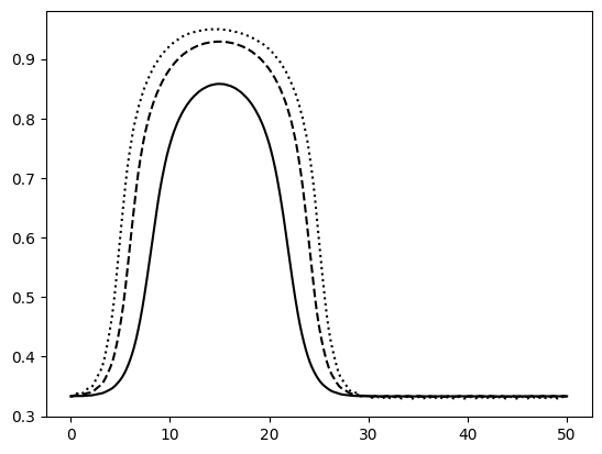
../_images/3f9764f939ee34c90321324bf920cc26b418da2d5d8a8f765618b7f6cb2f34ec.png

Stronger laser fields correspond to a higher degree of alignment, although this converges for large field strengths. The alignment is much stronger than in the non-adiabatic case, but at the cost of an external alignment field that may perturb molecular dynamics.

Alignment of an excited rotational state

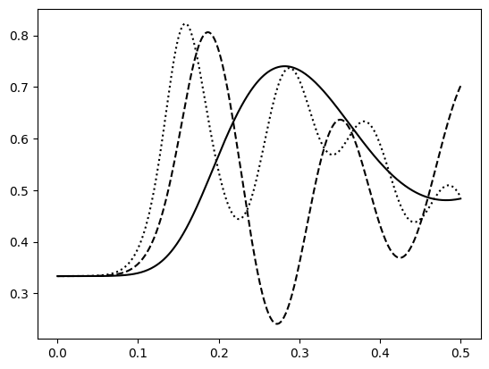
Finally, we can also study the alignment of rotationally excited states. A new feature in this case is that the magnetic quantum number “m” no longer needs to be zero. Let us reproduce figure 3 of ref.[1].

data = [calculate_alignment(Delta=400, sigma=0.05, l0=5, m=m) for m in range(6)]

times = data[0][0]
results = [vals for (t, vals) in data]

# factor of 2 because positive and negative m yield the same result
average = results[0]
for m in range(1,6):
    average = average + 2 * results[m]
average /= 11

plt.plot(times, average, '-k',
         times, results[0], '-.k',
         times, results[2], '--k',
         times, results[4], ':k');

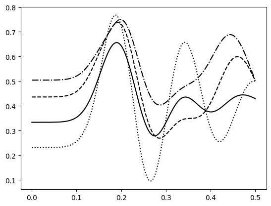
../_images/22ed321b8cd7e62bed23a7dc832cf032fad08e99a06e779529c9a7356a122773.png

The plot shows the average over all magnetic quantum numbers (solid line), and the individual results for m = 0, 2, 4 (dot-dashed, dashed, dotted line). While an increasing magnetic quantum number results in less field-free alignment, the total alignment is similar for all even values of m. The averaged alignment, however, is significantly damped, and smaller due to the lower alignment of odd values of m.