Background theory: Polynomial solvers

This web page can be downloaded as notebook: polynomial_solvers.ipynb (Jupyter) or polynomial_solvers.md (Markdown)

The usage of the most common Chebychev solver is documented in Using Chebychev solvers, see there on the practical aspects. Here, we want to give some more theoretical details on the subject for those inclined to dig deeper. In particular, we shall derive the formulas in a little more depth, discuss the magic values for the alpha number, and compare the performance of Chebychev solver to that of ODE solvers.

We will restrict the discussion to closed systems with real eigenvalues. The use of Chebychev polynomials was pioneered by Tal-Ezer and Kosloff [1]. It is possible to extend the treatment to purely imaginary eigenvalues, this is discussed in Ground-state relaxation and finite temperatures, and the original work [2]. An extension of the Chebychev method to arbitrary complex-valued systems (open systems, absorbing boundary conditions) was introduced by Huisinga et al. [3], but we omit this discussion for simplicity.

Basic theory

For a time-independent, closed system, the time evolution operator is defined by

$\psi(t+\Delta t) = \hat U(\Delta t) \psi(t) = \mathrm{e}^{-\imath \hat H \Delta t} \psi(t).$

Note

This and the following discussion also applies to density operators. Replace all operators by corresponding Liouvillians (operators in dual space) and the wave function by the density operator (state in dual space) and all arguments can be trivially translated.

The basic idea of polynomial solvers is to expand this exponential in a convenient series of classical polynomials. Complex Chebychev polynomials are used because of their superior convergence properties. Our first problem is that this polynomial series converges only in the interval [-i, i]. Translated appropriately, this means that the Hamiltonian must have all eigenvalues in the interval [-1, 1]. To get there, we first rescale the Hamiltonian,

$\mathrm{e}^{-\imath \hat H \Delta t} = \mathrm{e}^{-\imath (E_{\mathrm{min}} + \Delta E / 2) \Delta t} \mathrm{e}^{-\imath \alpha \hat H_\mathrm{norm}}$

where

$\begin{eqnarray*} \alpha =& \frac{\Delta E \ \Delta t}{2}\\ \hat H_\mathrm{norm} =& \frac{2}{\Delta E} (\hat H - E_\mathrm{min} - \frac{\Delta E}{2}) . \end{eqnarray*}$

Here, $E_\mathrm{min}, \Delta E$ denote the Hamiltonian’s smallest eigenvalue and the spectral range, respectively. It can be checked that the normalized Hamiltonian has all eigenvalues in the interval [-1, 1].

The first exponent is just a constant factor, and we only expand the second exponential with the normalized Hamiltonian and “time” $\alpha$ as

$\mathrm{e}^{-\imath \hat H_\mathrm{norm} \alpha} = \sum_{n=0}^N a_n(\alpha) \phi_n(-\imath \hat H_\mathrm{norm}),$

where up to constants, the coefficients “a” are Bessel functions of the first kind and the functions are the complex Chebychev polynomials.

Convergence

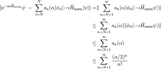
The huge advantage of Chebychev polynomials is the availability of an exact upper bound for the propagation error. We start with two inequalities, see [4], equations 22.14.4 and 9.1.62, which readily generalize to functions of operators:

$\begin{align*} |\phi_n(x)| =& |T_n(-\imath x)| &\leq 1 (x \in [-\imath, \imath]) \qquad \rightarrow \qquad \|\phi_n(-\imath \hat H_\mathrm{norm}) \psi\| \leq \|\psi\|\\ |J_n(x)| \leq& \frac{|x/2|^n}{n!} \end{align*}$

Now let us assume that we used the first N terms of the expansion and want to know the error when propagating a state. We get for a normalized state

$\begin{align*} \| \mathrm{e}^{-\imath \alpha \hat H_\mathrm{norm}} \psi \ - \ \sum_{n=0}^N a_n(\alpha) \phi_n(-\imath \hat H_\mathrm{norm}) \psi \| =& \| \sum_{n=N+1}^\infty a_n(\alpha) \phi_n(-\imath \hat H_\mathrm{norm} \psi)\|\\ \leq& \sum_{n=N+1}^\infty a_n(\alpha) \|\phi_n(-\imath \hat H_\mathrm{norm} \psi)\|\\ \leq& \sum_{n=N+1}^\infty a_n(\alpha)\\ \leq& \sum_{n=N+1}^\infty \frac{(\alpha/2)^n}{n!} \end{align*}$

We do not care about the exact value of the error, just note two properties of the expression:

There is an upper bound for the error independent of the initial state. That is, the convergence is continuous, there are no individual states for which the series does not converge.
For large enough N, the right-hand side decreases exponentially with increasing N.

In practice, we do not target a specific value of the (upper bound of the) propagation error, but simply truncate the series as soon as the Bessel function has reached a certain cutoff. This cutoff can still be considered a proxy for the order of magnitude of the error, but is not a rigorous quantity.

Efficiency of the Chebychev solver and good alpha values

Now we can finally discuss good alpha values for acceptable efficiencies. This discussion is very brief in the original papers.

The computational cost is essentially proportional to the order of expansion n; the Chebychev polynomials are calculated through a recursion relation, and each recursion requires one expensive evaluation of the Hamiltonian / Liouvillian. The order of expansion, that is, the cost, is defined by the Bessel functions dropping below a certain threshold. The size of the time step, that is, the gain, however, is proportional to the alpha value, i.e., the argument of said Bessel function.

So we can rephrase the question: At which value of alpha do we get most gain per cost? Let us plot the behaviour of the Bessel functions for different values of alpha

import matplotlib.pyplot as plt
import numpy as np
import scipy

alpha, n = np.meshgrid([20, 40, 60, 80], np.arange(120))
y = np.abs(scipy.special.jv(n, alpha))

fig, ax = plt.subplots()
ax.set_ylim(1e-12, 1)
ax.semilogy(n, y);

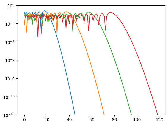
../_images/beb22fcf82e760d1b0167a65746802907a6a45cf748f01d253e7e41eff9cda51.png

We can clearly see that the Bessel functions are significant up to $n \approx \alpha$ , then they decay rapidly, approaching values of 1e-12 within roughly 30 orders. No matter our timestep, we always have to include these thirty orders to get a well-converged solution. Hence, a good alpha value should definitely not be smaller than about 30.

As an example, let us compare alpha values of 20 and 60. For the former, we need an order of 50, but our time step is shorter, and we need to step three times. Altogether that makes approximately 150 applications of the Hamiltonian. For the latter, we need a single time step with an order of 90, hence about 90 applications of the Hamiltonian. Thus, the latter alpha value requires only about 60% of the computing time of the smaller alpha value.

This gain starts to level off when alpha becomes larger than this constant decay. Hence, the proposition of using an alpha value of at least 40 to avoid inefficiencies, and there is little point of increasing alpha beyond, say, 100. Both values are not exact numbers, however, just crude rules of thumb.

However, very large orders of expansion may lead to artefacts. For example the values of the Bessel functions may become inaccurate, depending on the implementation details. Therefore, we would recommend not increasing alpha beyond something like 100, but that is also not a hard value. For example, we encountered a Matlab version around 2010 that would produce infinite solutions for large orders (200 or 300).

As a side note, the plot also shows that the precision has remarkably little influence on the efficiency. Even if we go for embarrassingly large values of 1e-6, the required polynomial orders are reduced only by about 10, which is why we use a fixed value of 1e-12 for the cutoff.

Comparison between Chebychev and ODE solvers

So far we have only claimed that the Chebychev solver is much faster than ODE solvers, so let us back this up with numbers. We choose the truncated harmonic oscillator example from Using Chebychev solvers.

import math
import wavepacket as wp

grid = wp.grid.Grid(wp.grid.PlaneWaveDof(-10, 10, 128))
psi0 = wp.builder.product_wave_function(grid, wp.special.Gaussian(-5, 0, rms=1))

kinetic = wp.operator.CartesianKineticEnergy(grid, 0, mass=1, cutoff=35)
potential = wp.operator.Potential1D(grid, 0, lambda x: 0.5 * x ** 2, cutoff=35)
equation = wp.expression.SchroedingerEquation(kinetic + potential)

First, we need to measure the speed. A good proxy is the number of times that our Hamiltonian is applied, because this is often the most expensive single operation. To count this value, we write a custom “counting expression” that just measures how often the solver calls it.

class CountingExpression(wp.expression.ExpressionBase):
    def __init__(self, wrapped_expression):
        super().__init__(False)

        self._wrapped_expression = wrapped_expression
        self.count = 0

    def apply(self, state, t):
        self.count += 1
        return self._wrapped_expression.apply(state, t)

Then we only wrap our (truncated) expression and propagate for a common time.

counting_equation = CountingExpression(equation)

solver_chebychev = wp.solver.ChebychevSolver(counting_equation, math.pi/2, (0, 70))
solver_chebychev.step(psi0, t=0)
print(f"Chebychev solver:                      count={counting_equation.count}, alpha={solver_chebychev.alpha:.4}")

counting_equation.count = 0
solver_rk45 = wp.solver.OdeSolver(counting_equation, math.pi/2)
solver_rk45.step(psi0, t=0)
print(f"Runge-Kutta 4/5 solver:                count={counting_equation.count}")

counting_equation.count = 0
solver_rk45_precise = wp.solver.OdeSolver(counting_equation, math.pi/2, rtol=1e-9, atol=1e-9)
solver_rk45_precise.step(psi0, t=0)
print(f"High-precision Runge-Kutta 4/5 solver: count={counting_equation.count}")

Chebychev solver:                      count=90, alpha=54.98
Runge-Kutta 4/5 solver:                count=404
High-precision Runge-Kutta 4/5 solver: count=1586

So even when comparing against a low-precision ODE solver (default 1e-6 for relative and absolute error of a single elementary time step), the Chebychev solver yields a factor of 4.5 in performance. If you require the higher precisions that you get for free with the Chebychev solver, simple ODE solvers are easily an order of magnitude slower.