Background theory: Converging equally-spaced grids
This web page can be downloaded as notebook: plane_wave_grid.ipynb (Jupyter)
or plane_wave_grid.md (Markdown)
When setting up a grid, you need to ensure that it can adequately represent the wave functions.
Failure to do so leads to inaccurate results or artifacts.
In this document, we want to dig a bit deeper, what happens when you choose an
inappropriate equally-spaced grid,
as encapsulated in wavepacket.grid.PlaneWaveDof.
In particular, we want to answer the questions:
What happens if the grid extension is too small for your dynamics?
How can you get away with less extension and fewer grid points?
What happens if you choose too few grid points?
Short recap: Equally-spaced grids and DVR
An equally-spaced grid is determined by three parameters:
The start of the grid  , the length
  , and the number of points
  .
The grid points are at
.
The grid points are at  with spacing
  and
and  .
This equally-spaced grid has a complementary,
equally-spaced grid in Fourier space with grid points
.
This equally-spaced grid has a complementary,
equally-spaced grid in Fourier space with grid points  in the interval
![[- \pi/\Delta x, \pi/Delta x]](../_images/math/d68f3ee22e39d6f2e66d006bfd9d760d1d12908e.png) .
The exact grid points are different for even and odd values of ,
but these minor details are not relevant for the subsequent discussion.
.
The exact grid points are different for even and odd values of ,
but these minor details are not relevant for the subsequent discussion.
The usage of this grid within the DVR approximation rests on three pillars:
Any wave function can be expanded in plane waves
 .
This expansion is the finite basis representation (FBR).
.
This expansion is the finite basis representation (FBR).The FBR contains the same information as if the wave function is given only at the grid points
 (discrete variable approximation, DVR).
This theorem is known as the Nyquist theorem in signal processing.
(discrete variable approximation, DVR).
This theorem is known as the Nyquist theorem in signal processing.Local operators such as potentials can be applied by multiplying the potential values at each grid point,
 \approx V(x_l) \psi(x_l)](../_images/math/94c73ce88328b8dbf2ffaef679c1c75c6cbfad08.png) .
This DVR approximation is exact if the result
.
This DVR approximation is exact if the result  is band-limited in
 ![[-K, K]](../_images/math/3c226d4a3b90400b68a9c0e4fc666dfa43527111.png) .
.
Effect of too small grid
Equally-spaced grids imply periodic boundary conditions.
If you expand a wave function in the FBR, you will find that  .
Choosing the grid too small causes the wave function to bleed into adjacent cells.
.
Choosing the grid too small causes the wave function to bleed into adjacent cells.
For a simple example, let us take a free particle and give it some final momentum:
import wavepacket as wp

dof = wp.grid.PlaneWaveDof(-20, 20, 128)
grid = wp.grid.Grid(dof)

kinetic = wp.operator.CartesianKineticEnergy(grid, 0, mass=1)
expression = wp.expression.SchroedingerEquation(kinetic)
psi0 = wp.builder.product_wave_function(
            grid, wp.special.Gaussian(x=0, p=3, rms=1))

solver = wp.solver.OdeSolver(expression, 4)
plotter = wp.plot.StackedPlot1D(4, psi0)
for t, psi in solver.propagate(psi0, 0, 3):
   plotter.plot(t, psi)
/home/docs/checkouts/readthedocs.org/user_builds/wavepacket/envs/stable/lib/python3.13/site-packages/wavepacket/plot/plot_1d.py:178: UserWarning: No artists with labels found to put in legend.  Note that artists whose label start with an underscore are ignored when legend() is called with no argument.
  axes.legend(loc="upper right")
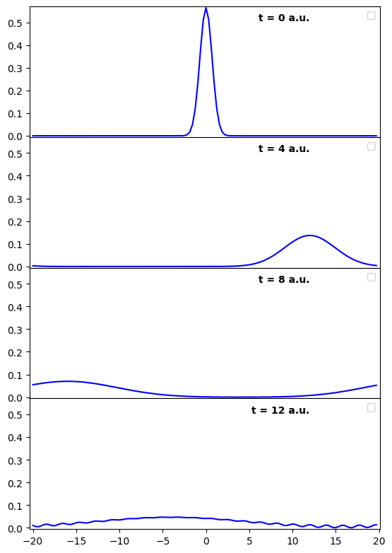
The initial Gaussian broadens and moves with positive velocity. As soon as it reaches the grid boundaries, it enters the grid from the opposite side due to the periodic boundary conditions. Also, in the last plot, the Gaussian has broadened so much that the right side (roughly corresponding to the components with the larger momentum) overtakes and interferes with the left side (roughly corresponding to components with smaller momentum). This results in an interference pattern, and these oscillations are also typical artifacts if the grid is chosen too small.
In practice, you often encounter reflection as another typical effect. For demonstration, let us dissociate an OH radical. We give the molecule strong initial kick as a crude simulation of dissociation.
import numpy as np

def morse_potential(x):
    r_e = 1.821
    alpha = 1.189
    D = 0.1994

    return D * (1 - np.exp(-alpha * (x - r_e)))**2


dof = wp.grid.PlaneWaveDof(0.7, 12, 256)
grid = wp.grid.Grid(dof)

kinetic = wp.operator.CartesianKineticEnergy(grid, 0, mass=1728.539)
potential = wp.operator.Potential1D(grid, 0, morse_potential)
equation = wp.expression.SchroedingerEquation(kinetic + potential)

shape = wp.special.Gaussian(x=1.4, p=35, rms=0.15)
psi0 = wp.builder.product_wave_function(grid, shape)

solver = wp.solver.OdeSolver(equation, dt=250)
plotter = wp.plot.StackedPlot1D(3, psi0, potential, kinetic+potential)
for t, psi in solver.propagate(psi0, 0.0, 2):
    plotter.plot(t, psi)
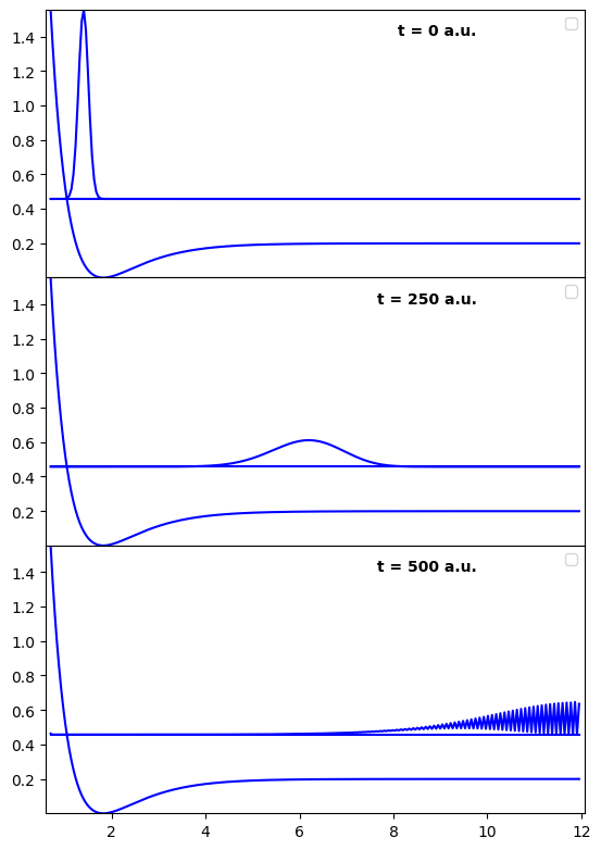
As the quasi-free wave packet reaches the end of the grid, it is reflected by the Coulomb barrier from the next periodic cell. The effect is again an interference between the outgoing and reflected parts of the wave packet, which shows up as rapid oscillations.
A problem that you may sometimes encounter is that your grid is always too small. Take the Morse oscillator example with a laser-driven dissociation of a molecule. The laser may be turned on for some time, and the simulation time must be longer than the laser pulse plus typical dissociation times. But during that simulation, the parts of the wave packet that dissociated first may reach the boundary of the grid, no matter how large it is chosen. In such a case, you probably want to use absorbing boundary conditions.
Absorbing boundary conditions
These conditions typically take the form of negative imaginary potentials (NIPs) [1] [2]. They can be used with any basis, but are usually needed for problems like molecular dissociation, for which a plane wave expansion / equally-spaced grid is most natural.
NIPs absorb the wave packet at the locations where they are nonzero, before the wave packet reaches the grid boundaries. There are, however, two major drawbacks:
If the potential is too large, the NIP itself can modify the dynamics. Consider a case where the NIP at some grid point absorbs effectively the whole wave packet in a small timestep. This effect is similar to an infinite potential wall, and may thus reflect the wave packet. A consequence is that you should choose the NIP to be as small and smooth as possible, and you may need to converge this as well.
With the NIP term, the Hamiltonian is no longer self-adjoint. Some efficient solvers like the ChebychevSolver only work for self-adjoint Hamiltonians. A possible workaround here is to move the NIP out of the Hamiltonian, and absorb the wave packet after every propagation step. As of Wavepacket 0.4, this is not implemented conveniently, though.
Let us demonstrate the first point by adding a steep NIP to the Morse oscillator example:
def bad_nip_potential(x):
    interval = np.ones(x.shape)
    interval[x < 8] = 0

    return -1j * interval * 10

bad_nip = wp.operator.Potential1D(grid, 0, bad_nip_potential)
equation = wp.expression.SchroedingerEquation(kinetic + potential + bad_nip)

solver = wp.solver.OdeSolver(equation, dt=150)
plotter = wp.plot.StackedPlot1D(3, psi0, potential, kinetic + potential)
for t, psi in solver.propagate(psi0, 0.0, 2):
    plotter.plot(t, psi)
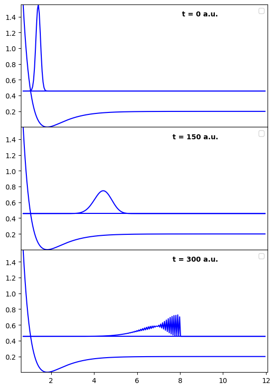
Our wave function is reflected at the start of the NIP around 8 a.u as predicted.
For a better approach, we can run a back-of-the-envelope calculation. Let us say that an OH distance of 8 atomic units is almost dissociated; any part of the wave function that gets there can be safely absorbed without perturbing the bound-states. Also, from studying the dynamics, it takes at least 100 atomic units for the shoulder to travel from 8 a.u. to the end of the grid at 12 a.u.
For a constant potential, the absorption of the density is roughly
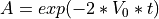 (the factor two comes because the absorption acts on the wavefunction
but the density is the square of the wavefunction).
If we aim to absorb 99% of the density (A = 0.01),
plugging in t=100 yields a value of V_0 approximately 0.025 a.u.
In practice, we might want to use a smooth turn-on (e.g., harmonic potential) that is zero at r = 8 a.u,
and about the intended value at r = 10 a.u.
Our final potential is then
(the factor two comes because the absorption acts on the wavefunction
but the density is the square of the wavefunction).
If we aim to absorb 99% of the density (A = 0.01),
plugging in t=100 yields a value of V_0 approximately 0.025 a.u.
In practice, we might want to use a smooth turn-on (e.g., harmonic potential) that is zero at r = 8 a.u,
and about the intended value at r = 10 a.u.
Our final potential is then  .
.
Let us plug this calculation into the Morse oscillator example from before:
def nip_potential(x):
    interval = np.ones(x.shape)
    interval[x < 8] = 0

    return -1j * interval * 0.025 / 4 * (x-8)**2

nip = wp.operator.Potential1D(grid, 0, nip_potential)
equation = wp.expression.SchroedingerEquation(kinetic + potential + nip)

solver = wp.solver.OdeSolver(equation, dt=150)
plotter = wp.plot.StackedPlot1D(5, psi0, potential, kinetic + potential)
for t, psi in solver.propagate(psi0, 0.0, 4):
    plotter.plot(t, psi)
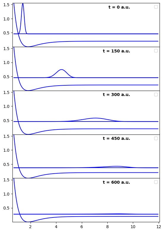
While the calculation may not have been the most sophisticated approach, it was good enough to smoothly absorb the wave function without artifacts. For additional refinement, we would have used this estimate as a starting point to tune the NIP parameters.
We have only scratched the surface of absorbing boundary conditions here, you can dig a lot deeper, e.g. [2] [3]. As usual, you should balance the gain against the invested time, though.
Effect of too few grid points
To quickly understand the effect of too few points for a given grid extent, we start with two observations:
The FBR is also an equally-spaced grid in momentum space. The extent of this grid is proportional to the inverse grid spacing / the number of grid points.
The transformation between the DVR and the FBR is a unitary Fourier transformation.
So instead of starting from zero, we transform our wave function into the FBR. Then we can wonder what happens if the equally-spaced FBR grid is too small for the wave function?. The answer, elaborated before, is that we have implicit periodic boundary conditions also in FBR, and our wave packet re-enters from the other side of the grid.
Let us study this effect for a Gaussian wave packet sliding down a linear ramp:
dof = wp.grid.PlaneWaveDof(-20, 20, 128)
grid = wp.grid.Grid(dof)

kinetic = wp.operator.CartesianKineticEnergy(grid, 0, mass=1)
potential = wp.operator.Potential1D(grid, 0, lambda x: -2 * x)
equation = wp.expression.SchroedingerEquation(kinetic + potential)

shape = wp.special.Gaussian(x=-10, p=0, rms=1)
psi0 = wp.builder.product_wave_function(grid, shape)

solver = wp.solver.OdeSolver(equation, 2.5)
plotter = wp.plot.StackedPlot1D(4, psi0, potential)
for t, psi in solver.propagate(psi0, 0.0, 3):
    plotter.plot(t, psi)
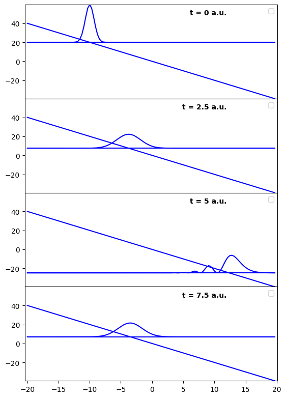
Initially, the wave packed moves down the linear ramp as we would expect. However, well before the end of the grid, something strange happens that makes the wave packet move up the ramp again.
What happens can be easily spotted if we plot the corresponding densities in FBR. This is currently not natively supported in Wavepacket, but we can write a stacked plot manually:
import matplotlib.pyplot as plt

figure, axes = plt.subplots(4, 1, sharex=True)
figure.subplots_adjust(hspace=0)
figure.set_figheight(figure.get_figheight() * 2)
index = 0

for t, psi in solver.propagate(psi0, 0.0, 3):
    x = grid.dofs[0].fbr_points
    y = wp.fbr_density(psi)

    axes[index].plot(x, y)
    index += 1
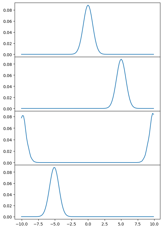
As predicted, the Gaussian wave packet gains momentum until it no longer fits inside the FBR grid. As soon as it reaches the boundary, then the wave packet enters from the other side, which corresponds to negative momenta. this causes unexpected interferences while the wave packet traverses the grid boundary, then the wave packet uses the negative momentum to ascend the ramp again.
Conclusion
If the grid extent is too small, you notice effects of periodic boundary conditions; wave packets are either reflected at the grid boundaries or enter the grid from the other side. If you cannot afford a large enough grid to avoid these periodic boundaries, you can work around most problems with a negative imaginary potential. Having too few grid points causes the same effects in Fourier space. These are easily spotted by monitoring the wave packet dynamics in the FBR.
Checking the convergence of an equally-spaced grid does not require sophisticated techniques; eyeballing is usually good enough. You should always monitor the wave packet dynamics in the DVR and the FBR.