Representing states at finite temperature
This web page can be downloaded as notebook: thermal_states.ipynb (Jupyter)
or thermal_states.md (Markdown)
Introduction
Sometimes, we wish to study systems at finite temperatures. To describe such systems, we need either a density operator or an ensemble of wave functions. The textbook expression for a thermal state is a density operator
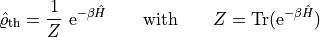
with the inverse temperature 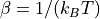 in terms of Boltzmann’s constant and the system temperature.
Note that we use atomic units throughout this text.
in terms of Boltzmann’s constant and the system temperature.
Note that we use atomic units throughout this text.
The thermal state itself is often not terribly interesting, but we want to calculate expectation values, typically the response to some perturbation,
(1)
To calculate the expectation value, we may have to evolve the density operator in time, for example under the influence of a laser field. As most of the subsequent discussion is focused on closed systems, we have represented the time evolution with a unitary operator here.
In this document, we present three different approaches for representing a thermal state and for calculating the response. For simplicity, we only calculate the temperature-dependent energy, but the path to more complex setups should be readily apparent from the formulas.
The system under study
As example system, we calculate the temperature-dependent energy of a Morse oscillator,
with parameters chosen for an OH radical.
The system is simple, but not entirely trivial.
Because we are going to use the RelaxationSolver,
we truncate the operators at energies well beyond the dissociation energy.
This has the side effect of providing us bounds for the spectrum of the Hamiltonian that we can use later.
import numpy as np
import wavepacket as wp

D_e = 0.1994;
r_e = 1.821;
alpha = 1.189;
mass = 1728.539

def morse_potential(x):
    return D_e * (1 - np.exp(-alpha * (x - r_e))) ** 2

dof = wp.grid.PlaneWaveDof(0.7, 7, 128)
grid = wp.grid.Grid(dof)

hamiltonian = (wp.operator.CartesianKineticEnergy(grid, 0, mass=mass, cutoff=1)
               + wp.operator.Potential1D(grid, 0, morse_potential, cutoff=1))

# useful for later setups
spectrum = (0, 2)
beta_vals_to_calculate = [100, 25, 10]
Note that the chosen temperatures are high, well above thousand Kelvin. They should not be understood as examples of typical physics, but as numerical examples corresponding to different regimes:
For beta = 100 (
 is 1/20th of D_e),
the temperature is on the order of the excitation energy.
is 1/20th of D_e),
the temperature is on the order of the excitation energy.For beta = 25 (
is 1/5th of D_e),
the temperature is larger than the excitation energy, and significant compared to the dissociation energyFor beta = 10 (
is 1/2 of D_e),
the temperature is on the order of the dissociation energy
Method I: Using the thermal density operator directly
Theory
The first approach directly constructs the thermal density operator,  .
The exponentiation is difficult, therefore we use a roundabout way also described in Ground-state relaxation and finite temperatures.
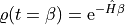
It can be checked that, the initial-value problem
.
The exponentiation is difficult, therefore we use a roundabout way also described in Ground-state relaxation and finite temperatures.
It can be checked that, the initial-value problem
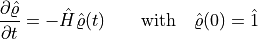
has the solution
which is exactly our thermal density operator except for the trivially calculated normalization factor.
The differential equation is solved by the wavepacket.solver.RelaxationSolver, so we only need to
prepare the initial state and let the solver run.
Implementation
The implementation closely follows the theory. We propagate the state and calculate the corresponding expectation values.
for beta in beta_vals_to_calculate:
    solver = wp.solver.RelaxationSolver(hamiltonian, beta, spectrum)

    unit_density = wp.builder.unit_density(grid)
    rho = solver.step(unit_density, 0)
    Z = wp.trace(rho)

    thermal_state = wp.normalize(rho) # or you divide by Z
    energy = wp.expectation_value(hamiltonian, thermal_state).real

    print(f"beta = {beta}: Z = {Z:.4}   energy = {energy:.4}")
beta = 100: Z = 0.5005   energy = 0.01281
beta = 25: Z = 2.605   energy = 0.05202
beta = 10: Z = 9.503   energy = 0.1396
Note that the solver is rather inefficient due to the mostly small alpha values, but in practice this would not matter. You prepare the initial state once, and any time evolution dwarves the cost of the relaxation. If you do not need the partition sum explicitly, you can avoid its calculation by directly normalizing the resulting density operator.
Conclusions
The calculation of a thermal density by imaginary-time propagation is straight forward. It has a direct connection to the theory, where the density-operator formalism is common. Finally, the implementation is simpler than for the alternative methods.
If you want to study open systems, you probably want a density operator to describe interactions with the environment, so this approach ties in perfectly. If, however, you study closed systems, density operators can be awkward. Also, if we look beyond the scope of this humble Python package, density operators might simply not be available, for example if you use MCTDH for large systems.
Consider a system of N total grid points / basis functions. To represent a density operator, you need to store N^2 values, compared to N values for a wave function. The cost of applying an operator is somewhere between pointwise multiplication (potentials in DVR approximation) and matrix multiplication (general, unoptimized operator). For a density operator, this computational cost scales between N^2 to N^3, while for wave functions the scaling is between N and N^2.
As a result, density operators are only applicable for rather small systems, otherwise the memory requirements will kill you. And their propagation in time is comparably slow compared to that of a small ensemble of wave functions. So if we do not need a density operator, we may want to avoid it. That is what the other approaches do.
Method II: Using eigenstates of the Hamiltonian
Theory
To motivate the use of energy eigenstates, let us use the cyclic property and the definition of the trace to rewrite the (1).
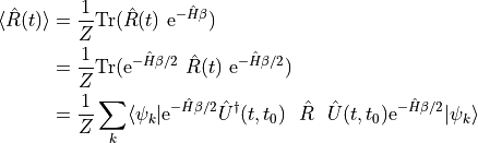
This equation directly suggests an alternative procedure for calculating thermal averages:
Choose some orthonormal basis.
For each basis function, first do an imaginary-time propagation up to half the inverse temperature, then propagate in real time up to the point where the observable is calculated.
For each such propagated wave function, calculate the expectation value, and sum up all the results.
Divide the sum by the partition sum. From its definition, we formally get the partition sum by calculating steps 1-3 with the unit operator as response.
Note that this procedure is applicable to every orthonormal basis. So, with some algebra, we succeeded in replacing the density operator by an ensemble of wave functions. This helps with memory requirements, because we only need to store one or few wave functions at a time, but does not improve performance. While a single wave function is faster to propagate, we need to do so for the full basis of N wave functions, which turns out to be as expensive as propagating the density operator.
As a consequence, this scheme makes most sense if we can faithfully reproduce the results using only few of the basis functions. Hence, we need a basis where the result converges (exponentially) quickly, and one such set are the eigenfunctions of the Hamiltonian. We find that
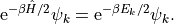
For energies 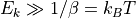 , the exponential term becomes negligible,
and the eigenstate does not matter for the result.
For sufficiently low temperatures, few eigenstates suffice, making this scheme rather efficient.
A further convenient benefit of energy eigenstates is that the exponential term is a number, and we need no
explicit solver.
, the exponential term becomes negligible,
and the eigenstate does not matter for the result.
For sufficiently low temperatures, few eigenstates suffice, making this scheme rather efficient.
A further convenient benefit of energy eigenstates is that the exponential term is a number, and we need no
explicit solver.
Implementation
For simplicity, we choose to obtain the eigenstates here from diagonalising the Hamiltonian matrix. This is not a good choice performance-wise, but keeps the example focused.
Conceptually, we need two passes. In a first pass, we calculate the partition sum, then we can calculate the expectation values of the response operator. In practice, the partition sum can be trivially obtained from intermediate results.
energies_and_states = [val for val in wp.diagonalize(hamiltonian)]

for beta in beta_vals_to_calculate:
    print("++++++++++++++++++++++++++++++++++++++++++++++++++++++")
    print(f"beta = {beta}")

    for num_states in [2, 4, 16, 64]:
        ensemble = energies_and_states[:num_states]

        Z = 0
        response = 0

        for energy, psi in ensemble:
            relaxed_state = np.exp(-energy * beta / 2.0) * psi

            Z += wp.trace(relaxed_state)
            response += wp.expectation_value(hamiltonian, relaxed_state).real

        print (f"N={num_states}:   Z = {Z:.4}    E = {response / Z:.4}")
++++++++++++++++++++++++++++++++++++++++++++++++++++++
beta = 100
N=2:   Z = 0.4825    E = 0.01154
N=4:   Z = 0.4996    E = 0.01269
N=16:   Z = 0.5005    E = 0.01281
N=64:   Z = 0.5005    E = 0.01281
++++++++++++++++++++++++++++++++++++++++++++++++++++++
beta = 25
N=2:   Z = 1.32    E = 0.01572
N=4:   Z = 1.898    E = 0.02583
N=16:   Z = 2.498    E = 0.04502
N=64:   Z = 2.605    E = 0.05202
++++++++++++++++++++++++++++++++++++++++++++++++++++++
beta = 10
N=2:   Z = 1.684    E = 0.01681
N=4:   Z = 2.896    E = 0.03061
N=16:   Z = 6.207    E = 0.0797
N=64:   Z = 9.431    E = 0.1362
If we compare these values to the exact results for the density operator, we see a few trends.
Even for the lowest temperature, we need to include several excited states;
with four states we still have a residual error of about 1%.
For larger temperatures the thermal excitations are similar in magnitude to the binding potential,
and we need many more states for converged results.
An intuitive explanation is that as soon free or quasi-free states start to contribute,
there are a lot of them, and they compensate their small weights with sheer numbers.
Conclusions
The method based on energy eigenstates can have superior efficiency compared to the density operator approach for a moderate increase in conceptual complexity. For that reason, you will find it widely adopted in the literature. However, it has two mighty limitations: you need to converge with few enough states, and you need an efficient method to determine these states. The principal feasibility of this scheme can usually be checked with back-of-an-envelope calculations and a few test propagations, but you should still always monitor the convergence.
The cost scales with the number basis functions that you need.
As soon as the thermal excitation probability  becomes relevant for weakly-bound
states, convergence becomes expensive.
Hence, this approach is most useful for low temperatures with on the order of the
smallest excitation energy or less.
This situation is rather common for molecular vibrations and typical experimental conditions.
becomes relevant for weakly-bound
states, convergence becomes expensive.
Hence, this approach is most useful for low temperatures with on the order of the
smallest excitation energy or less.
This situation is rather common for molecular vibrations and typical experimental conditions.
Determining the eigenstates and -energies through diagonalizing the Hamiltonian, as we did here, is usually out of question; memory and computations are similar to those of the density approach of Method I. You are probably better off sticking to the accurate density-operator formalism than blindly adding complexity.
One solution is the use of imaginary-time relaxation to get the lowest few eigenstates. This method is discussed in Ground-state relaxation and finite temperatures. Curiously, the relaxation limitation to few excited eigenstates aligns naturally with the this method’s limitation to few excited eigenstates.
If relaxation is difficult, you can simply choose a different basis. After all, we do not need energy eigenstates, we need to cover the relevant low-energy subspace. As an example, take a rotating, vibrating molecule: Calculating the ro-vibrational eigenstates is tricky, but calculating the rotational or vibrational eigenstates is easy. So you might just construct your basis from products of rotational and vibrational eigenstates, which should give good enough coverage of the relevant energy range, and accept the residual systematic error. Note, though, that you need to relax these basis functions before the real-time evolution, because they are no longer true eigenstates of the Hamiltonian.
Method III: Using random wave functions
Theory
The derivation is similar in spirit to Method II, but instead of an orthonormal basis, we use special random wave functions [1][2],
![|\tilde \psi\rangle = \sum_k \tilde c_k |\psi_k \rangle
\qquad \mathrm{where} \quad E[\tilde c_k \tilde c_l^\ast] = \delta_{kl}
.](../_images/math/eb542b898dc4558300437af9c62abc3318c3aae3.png)
Note: We use the notation from our own publication[3], which may be a bit uncommon. The tilde denotes random quantities (variables, wave functions, operators). We get the random wave function by assigning a random number as coefficient of each basis function. The coefficients are normalized and uncorrelated. Roughly the only useful operation on a random variable is the calculation of the expected value, denoted “E[]”, which returns a “normal” number or object. The expected value calculation trivially commutes with non-random factors, and for practical applications boils down to an ensemble average.
With this setup, the projection operator becomes the normal unit operator under averaging,
![E[ |\tilde \psi \rangle \langle \tilde \psi | ]
= E[ \sum_{k,l} \tilde c_k \tilde c_l^\ast | \psi_k \rangle\langle \psi_l |]
= \sum_{k,l} E[\tilde c_k \tilde c_l^\ast] |\psi_k \rangle \langle \psi_l|
= \sum_k |\psi_k \rangle \langle \psi_k |
= \hat 1
.](../_images/math/fc5547152b9adfa6d7da54e8f4d1589dc23a76be.png)
Note
Random wave functions are only useful for certain manipulations, such as replacing a unit operator. You must not confuse them with ordinary wave functions, as not all operations are well-defined. For example, it is easy to check that they do not have a finite norm.
We now take again (1), split the exponential, insert and expand a unit operator, rearrange the scalar products, and finally use the resolution of identity to get rid of the trace summation,
![\begin{align*}
\langle \hat R(t) \rangle &= \frac{1}{Z} \ \sum_k \langle \psi_k | \hat R(t)
\mathrm{e}^{-\hat H \beta/2} \ \hat 1 \ \mathrm{e}^{-\hat H \beta/2}
| \psi_k \rangle
\\
&= \frac{1}{Z} \ E[ \langle \tilde \psi| \mathrm{e}^{-\hat H \beta/2}
\ \sum_k |\psi_k\rangle\langle\psi_k| \ \hat R(t)
\mathrm{e}^{-\hat H \beta/2} |\tilde \psi \rangle ]
\\
&= \frac{1}{Z} \ E[ \langle \tilde \psi \mathrm{e}^{-\hat H \beta/2} \hat U^\dagger(t, t_0)
\ \hat R \ \hat U(t, t_0) \mathrm{e}^{-\hat H \beta/2} |\tilde \psi \rangle ]
\end{align*}](../_images/math/3ce41b60d5a9f59ef8be956ef01dd71efdfbf205.png)
Similar to the previous discussion, this formula suggests a simple algorithm for calculating the response:
Generate an ensemble of random wave functions (with normalized, uncorrelated coefficients). More on that in a moment.
For each random wave function, propagate for half the inverse temperature in imaginary time.
Propagate the result in real time as required, and calculate the expectation value of the response operator.
Calculate the ensemble average of the expectation values.
Divide the average by the partition sum. The partition sum is calculated using steps 1 to 4 with a unit operator as response.
On first view, this method may look like a slightly deranged variant of the previous method II. So how, and especially why and when does it work? The hand-waving answer is that this is almost method II, but the ensemble of random wave functions (i) is not orthogonal (bad), and (ii) covers the “typical” Hilbert space space with few wave functions already (good).
Non-orthogonality is uniformly bad; it means for example that you may count contributions twice, and this problem only averages out over large samples. The coverage can be advantageous; instead of requiring many rigorous basis functions, you just construct a coherent superposition of many and get “all results in one go”. Depending on the relative importance of these two factors, the results may be terrific or terrible. Practice and even more diffuse hand waving suggests the former.
The final bit of theory concerns the construction of the random wave functions.
A convenient basis is the DVR; that is, we just assign a random coefficient to each grid point.
This saves additional transformations.
Then, we only need any scheme that is uncorrelated and normalized,
![E[\tilde c_k \tilde c_l^\ast] = \delta_{kl}](../_images/math/79c8f98d3a959e3a6941abf313271205eecc9bd8.png) .
A simple scheme assigns each coefficient a complex number
.
A simple scheme assigns each coefficient a complex number  where the phase is drawn uniformly from the interval
 ![\phi \in [-\pi, \pi]](../_images/math/613e125c0e6358458f7a1b118a5eddf4f7616440.png) .
.
Implementation
The overall implementation is similar to that of method II with three differences.
Instead of calculating eigenstates, we generate random wave functions using
wp.builder.random_wave_function().We need to explicitly relax the states.
We do not sum the individual contributions, but average.
rng = np.random.default_rng(42)

for beta in beta_vals_to_calculate:
    print("++++++++++++++++++++++++++++++++++++++++++++++++++++++")
    print(f"beta = {beta}")

    solver = wp.solver.RelaxationSolver(hamiltonian, beta/2, spectrum)

    for num_states in [1, 2, 4, 16, 64]:
        Z = 0
        response = 0

        for n in range(num_states):
            psi_0 = wp.builder.random_wave_function(grid, rng)
            relaxed_state = solver.step(psi_0, 0)

            Z += wp.trace(relaxed_state) / num_states
            response += wp.expectation_value(hamiltonian, relaxed_state).real / num_states

        print (f"N={num_states}:    Z = {Z:.4}    E = {response / Z:.4}")
++++++++++++++++++++++++++++++++++++++++++++++++++++++
beta = 100
N=1:    Z = 0.3032    E = 0.01227
N=2:    Z = 0.1839    E = 0.01957
N=4:    Z = 0.4767    E = 0.01192
N=16:    Z = 0.5722    E = 0.01353
N=64:    Z = 0.5464    E = 0.01257
++++++++++++++++++++++++++++++++++++++++++++++++++++++
beta = 25
N=1:    Z = 3.782    E = 0.04141
N=2:    Z = 2.97    E = 0.04946
N=4:    Z = 3.021    E = 0.04975
N=16:    Z = 2.586    E = 0.0527
N=64:    Z = 2.497    E = 0.05114
++++++++++++++++++++++++++++++++++++++++++++++++++++++
beta = 10
N=1:    Z = 9.445    E = 0.1478
N=2:    Z = 9.82    E = 0.1363
N=4:    Z = 10.51    E = 0.1387
N=16:    Z = 9.797    E = 0.1377
N=64:    Z = 9.726    E = 0.1375
Comparison against the exact results from the density operator (method I) demonstrates the good and the ugly. With a single random wave function, the results are already pretty good, with only a few 10% deviation even for the largest temperatures. On the other hand, even for 64 random wave functions, we have residual errors on the order of single percent.
Discussion
The implementation demo already shows the good parts of random thermal wave functions. You can get reasonable results very cheaply. This is also a finding in the literature. [1][2] [3][4] You get pretty good results already with ensembles of ten or even fewer random wave functions. And the results are uniformly ok for very different temperatures.
There are two caveats, though.
One is rather theoretical: Pseudo-random number generation even in 2025 is not a solved problem, all existing generators have issues. It is unlikely, but principally possible that your “random” numbers are less random than you think. Such problems are difficult to notice, let alone debug for a non-expert, so the only advice is to be critical of your results.
More severely, you get good results, but not converged results. With random wave functions, once you have added enough functions to reasonably sample the relevant subspace, you get stochastic convergence, and the relative error drops with the square root of the number of wave functions. Contrast this with the rigorous method II with energy eigenstates: It may be infeasible, but once you have sampled the relevant subspace, you get at some point exponential convergence.
This suggests that you want to monitor the fluctuations of the calculated response. Once the results do not improve significantly, you stop. Adding more functions will not improve the accuracy of your solution significantly, only the cost.