Schrödinger cat states
This demo demonstrates one of the core features of Wavepacket: Switching between wave functions and density operators with minimal overhead
We consider a simple free particle as a coherent or incoherent sum of two Gaussians. This shows the main features without too much detracting physics.
General setup
We start with a few convenience imports and shortcuts
import math

import matplotlib.pyplot as plt
import numpy as np
import wavepacket as wp
Both descriptions, wave function and density operator, share the grid, and the operator structure, so we only need to set it up once.
degree_of_freedom = wp.grid.PlaneWaveDof(-15, 15, 128)
grid = wp.grid.Grid(degree_of_freedom)
hamiltonian = wp.operator.CartesianKineticEnergy(grid, dof_index=0, mass=1.0)
Wave functions
For wave functions, we set up an initial wave function,
and create a Schrödinger equation,
 ,
that we then solve.
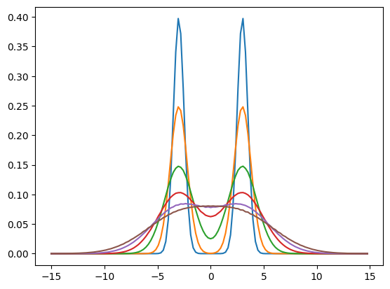
The overall dynamics are not spectacular:
The initial Gaussians only broaden over time.
,
that we then solve.
The overall dynamics are not spectacular:
The initial Gaussians only broaden over time.
In the plots, note the small peak in the density around the zero coordinate, and some wiggles as soon as the two wave functions come into contact with each other. Both features arise from the coherent addition of the two wave functions
rms = math.sqrt(0.5)
psi_left = wp.builder.product_wave_function(grid, wp.Gaussian(-3, rms=rms))
psi_right = wp.builder.product_wave_function(grid, wp.Gaussian(3, rms=rms))
psi_0 = math.sqrt(0.5) * (psi_left + psi_right)

schroedinger_eq = wp.expression.SchroedingerEquation(hamiltonian)
solver = wp.solver.OdeSolver(schroedinger_eq, dt=math.pi/5)

for t, psi in solver.propagate(psi_0, t0=0.0, num_steps=5):
    # TODO: Better and more convenient plotting
    plt.plot(grid.dofs[0].dvr_points, wp.grid.dvr_density(psi))
Density operators
For the equivalent density operator description, we have to set up the initial state
as a density operator. Here, we choose an incoherent summation of the two Gaussians,
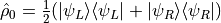 .
Also, the equation of motion is now a Liouville von Neumann equation (LvNE),
.
Also, the equation of motion is now a Liouville von Neumann equation (LvNE),
![\frac{\partial \rho}{\partial t} = \mathcal{L}(\hat \rho) = [\hat H, \hat \rho]_-](../_images/math/596cf3c6da4924219843ff5918f860b1605f9cdc.png) .
Note that both the Schrödinger equation and the LvNE contain the same
Hamiltonian, so we can recycle it.
.
Note that both the Schrödinger equation and the LvNE contain the same
Hamiltonian, so we can recycle it.
Besides these unavoidable changes, the interface works the same
as for the wave function case.
wavepacket.grid.dvr_density() in particular works for both types of states.
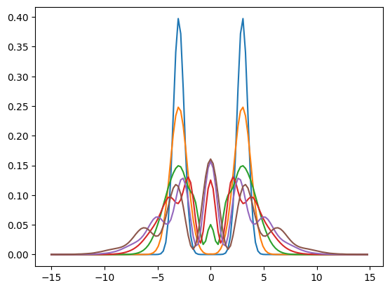
Note how the small peak at the zero coordinate and the wiggles are gone now.
This is the effect of the incoherent summation;
there is no coherence between the left and right Gaussian.
Had we chosen a coherent summation,
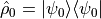 ,
we would have obtained the same result as for the wave function case including
the interference spike at
,
we would have obtained the same result as for the wave function case including
the interference spike at  .
.
rho_0 = 0.5 * (wp.builder.pure_density(psi_left) + wp.builder.pure_density(psi_right))

liouvillian = wp.expression.CommutatorLiouvillian(hamiltonian)
solver = wp.solver.OdeSolver(liouvillian, dt=math.pi/5)

for t, rho in solver.propagate(rho_0, t0=0.0, num_steps=5):
    # TODO: Better and more convenient plotting
    plt.plot(grid.dofs[0].dvr_points, wp.grid.dvr_density(rho))